

|
Вид публикации: Статья Год: 2013 Издательство: QUARTERLY JOURNAL OF INTERNATIONAL AGRICULTURE – В ПЕЧАТИ Целевое назначение: Научное Автор(ы): EKATERINA GATAULINA. HEINRICH HOCKMANN AND ANTON STROKOV Статус: завершенный Наименование: RISK. TECHNICAL EFFICIENCY AND MARKET TRANSACTION COSTS IN DIFFERENT ORGANISATIONAL FORMS: EVIDENCE FROM TATARSTAN AND OREOL Ключевые слова: risk production function, Russia, agroholdings Объем (п.л.): 1.1 Формат: обычная PDF-файл: http://www.viapi.ru/download/2013/126822.pdf |
Ekaterina Gataulina, Heinrich Hockmann, Anton Strokov.
Production Risk, Technology and Market Access in Different Organisational Forms: Evidence from Tatarstan and Oryol // Quarterly Journal of International Agriculture - №4/14. Vol. 53 (2014), No. 4: pp. 293-318
Abstract
This paper examines price and technology differentials between agroholdings and
independent farms in two Russian regions: Oryol and Tatarstan. Both
organisational forms receive on average the same product prices which indicates
that they have the same market access. Moreover, their technologies are also
very similar, as estimated by a risk production frontier. However, differences
in the factor input between organisational form lead to differences in the
shadow prices of the inputs, resulting from the better access of agroholdings
to the input markets. The results suggest that production risk, conditions on
the product market and inefficiency significantly affect agricultural
production. Thus, to improve the conditions, agricultural policy is required to
tackle all the issues in parallel using a mix of appropriate policy measures.
Keywords: risk production function, Russia, agroholdings
JEL: Q110, D220, P230
Vol. 53 (2014), No. 4: 293-318
1 Introduction
Several studies have revealed that Russia's agricultural sector is lagging behind the development of other sectors of the economy (Voigt and Hockmann 2008). The reasons for this phenomenon are intensively discussed among economists and politicians. In this paper we will contribute to this debate and analyse the significance of price and quantity risk as well as their influence on agricultural development and performance. The analysis will be conducted for the Tatarstan Republic and the Oblast Oreol. Agriculture in these two regions is subject to massive administrative support, especially regarding the support of agroholdings. Thus, it is interesting to identify how these political interventions may have contributed to agricultural development in these regions. In this context we will analysis prices as well as input and output have developed by organisational forms and how these indicators have influenced performance.
Analysing the variation of prices among farms provides information about market access. Thus, it provides information whether organisational forms have different access to markets (higher expected price) and whether the market conditions are mode stable (variation of proves). Quantity changes are due to production risk and technical inefficiency. Production risk leads to a variation of agricultural production around the average. This component basically results from the variation of natural conditions, e. g. weather. Technical inefficiency determine the degree to which producers are able to exploit production possibilities These indicators will be investigated for different organisational forms in order to assess whether productivity differences among agricultural enterprises are determined by the choice of technology or basically by ownership and governance structures in agricultural enterprises. Thus we will also contribute to the question whether the occurrence of horizontally and vertically integrated structures (often called agroholdings or business groups) have had a positive effect on agricultural production.[1] Moreover, we will identify which kinds of obstacles are mainly reduced when a farm becomes a member of an agroholding.
The central indicator in our analyses is revenue. In a first step we decompose its revenue variation into the variation of product prices and the variation of production. While the variation of product prices can be directly taken from the data. The contribution of the variation of production and it components (technology, production risk, ineffciency) has to be estimated using econometric techniques. In the second step, we therefore apply stochastic frontier analysis to determine how technology, risk and inefficiency affect agricultural production.
The paper is organised in six chapters. The next chapter presents some indicator for the agricultural sector in the two regions. Chapter 3 deals with the decomposition of the variance of revenues into the contribution of prices and quantities. Differences in the level of production (productivity) will also be investigated. Chapter 4 discusses the theoretical background used for the stochastic frontier analysis. It follows a discussion of the data used in the analysis. The results are presented in Chapter 5 where we discuss estimation results and the implication of the contribution of technology, risk and inefficiency to production. In Chapter 6, the findings from Chap. 3 and 5 are put together resulting in a coherent picture of the impact of market access, technology, risk and inefficiency.
2 Regional Characteristics
Oreol oblast is located in the southwest of Central Russia and Tatarstan is a part Volga District. Oreol oblast is 24.7 thousand km2, Tatarstan is almost 3 times bigger – 67.8 thousand km2. This finds its expression in the cultivated area which is also three times larger in Tatarstan than Oreol (2.5 against 0.8 m ha, respectively in 2008). Both regions have good weather and soil conditions for crop production (grains, potato, sugar beet) and extensive grassland for livestock breeding.
2.1 Agricultural development
After 2000 both regions experienced a strong increase in agricultural production (Figure 1). Between 2000 and 2011 gross agricultural output increase by almost 4% and more 5% p. a. in Oreol and Tatarstan, respectively. While in Tatarstan output growth begun already in 2000, the increase in Oreol started basically in 2007. In 2010, due to the blasts resulting from the extreme draught both regions experienced a sharp decline in output.
Surprisingly, the change in production was not accompanied by a similar development of input use in agriculture. In fact, except capital, all inputs are a lower level in 2011 compared to 2000. Regarding industrial inputs like capital and materials, the lowest level occurred in the middle of the decade. however, in recent years the use of these inputs started to increase in both regions. Like industrial inputs labour use in agriculture declined until the middle of the decade. After 2005 labour stabilized on a level about 25% lower than that of 2000 in both regions. The most remarkable difference between the regions concerns land input. While in Oreol land use went steadily down, the use of land in Tatarstan remained stable over the whole period.
Figure 1: Development of production and factor use, 2000-2011 (2000 = 1)
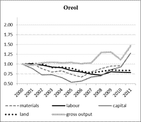
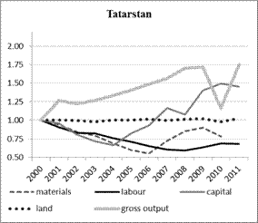
Soruce: own calculations based on Rosstat
The reasons for these developments itself as well as the difference between the regions are manifold. Explaining them in detail would go beyond the scope of this paper, however, two aspects should at least be mentioned: First, the reduction of inputs and the increased in output imply that technological change had played in important role in agriculture. This issue will be taken up later in Section 5 in more detail. Second, the agricultural sectors may have been subject to different intensities of support from the local and federal governments.
2.2 Agricultural policy
Exact figures which provide comprehensive information on policy intervention from the regional and federal government were not available, however, the share of subsidies on the value of production gives at least some information on the issue.
Figure 2: The relation between subsidies and the value of agricultural production, %
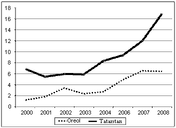
Source: Rosstat, Russian Ministry of Agriculture
One average public support for agriculture in terms of its share on the value of production was double as high in Tatarstan than in Oreol. Moreover, in recent years in Tatarstan the farms experienced a higher increase of subsidies than those in Oreol. One of the reason concerns the availability of funds. Tatarstan is an oil producing regions which benefited strongly from the increase in crude oil prices between 2000 and 2011. However, the scope of the subsidies programmes in the 2000-2008 period were rather similar in both regions: subsidies for buying fertilizers and feedstuff, subsidies for growing particular crops or grazing livestock, pig or poultry, compensation for interest rate. Moreover, in both region farms received public support for investment. The effects were massive investment in agriculture (see Figure 1). In the period from 2006 to 2008 farm in Tatarstan invested more the 50 bn Roubles in fixed assets. The figure for Oreol was only 17 bn Roubles.
Both regional governments fostered the creation of agroholdings. Starting in 1990, Oreol was one of the first regions were the government directly practiced the creation of vertically integrated structures. Basically two highly vertically, horizontally and diagonally integrated structures were formed which were strongly controlled by the regional and local governments.[2] The holdings had closed commodity chains, joint production planning as well as financial administration. Their purpose was not only agricultural but more generally rural development. Due to lack of effectiveness and profitability, at the end of the decade one of the big holdings (Orlovskaya niva) collapsed into several smaller vertically integrated agroholdings which specialized in sugar, grain, poultry and/or pork production and processing (Wandel 2010).
In the 1990’s Tatarstan was one of the regions that tried to save the former organizational forms – kolkhoz and sovkhoz – typical for Soviet Union. In the 2000’s the paradigm of agricultural policy changed and the creation of huge horizontally integrated structures was strongly supported. For instance, milk producing farms with 800-1500 cows on average and farms specialising on crop production which cultivate about 400 thousand ha per holding were established. As a result, 60% of the 2.5m ha available in that region were cultivated by the four largest agroholdings.
In the late 2000s both regions faced similar problems. First, since the holding were highly indebted, the companies suffered strongly from the financial crises. In addition, the regional governors who supported the holdings had left their positions. Some holdings might have lost state support and might have experienced problems in getting new credits.
3 quantity and price variation
3.1 Data
We use accountancy data of agricultural enterprises in Tatarstan Republic and Oblast Oreol for the period of 2006-2008 (Rosstat data provided by VIAPI). The original data sets contain about 1000 and 600 observations for Tatarstan and Oreol, repectively. First, we excluded observations with nonsense partial productivities, e. g. when land productivity or milk production per cows was 10 time larger than average. Second, we excluded farms for which we had only one observation. Including these would have led to large changes in the data sets in the individual years, and the entering and exiting of farms would have biased the results significantly. This cleaning provided resulted in data sets with 634 and 352 observations for Tatarstan and Oreol, respectively. In Tatarstan we have 238 independent farms and 40 holdings[3]. The numbers for Oreol are 148 and 24.
The data sets provides detailed information on production structures, specialisation and factor input. Moreover, implicit firm specific product prices can be calculated from the data set using the quantities and sales of marketed products. In a first step, we took a closer look at production and product prices of the agricultural enterprises. Our data set allows conducting comparable analyses for grain and milk. In order to assure that the comparisons are not biased by farm size, gross production was divided by an input unit. This unit represents the area planted with the corresponding crop and the number of cows in milk production. We first reveal information about different price and partial productivity structures of agroholding members and independent farms. In addition, we decompose the variance of output specific revenues in order to identify whether revenues by organisational form are differently affected by quantity and price variation.
3.2 Prices and partial productivities
Table 1 provides information about partial productivities and prices received by farmers. The data show that in neither region marked price differences between organisational structures existed. Basically, the same holds true for partial productivites. The results are quite astonishing. Often it is argued that prices received by holding members are only transfer prices and independent of market prices. The information in Table 1 provides no support of this view. This precludes that agroholdings conduct special price strategies and the result presented in Table 1 is incidental only. This could be investigated further by comparing prices between different agroholdings, however, these information is not available in the data. Although not as informative as holding specific prices, price variation between independent farms and group members may help to shed some light on this issue.
Table 1: Expected prices and quantities (per hectare)
|
Tatarstan |
|
Independent farms |
|||||
|
2006 |
2007 |
2008 |
|||||
|
E(y) |
E(p) |
E(y) |
E(p) |
E(y) |
E(p) |
||
|
Grain |
25.3 |
2.6 |
25.7 |
3.8 |
33.7 |
4.4 |
|
|
Milk |
35.9 |
5.8 |
37.9 |
7.0 |
41.7 |
8.9 |
|
|
|
Holding members |
||||||
|
2006 |
2007 |
2008 |
|||||
|
E(y) |
E(p) |
E(y) |
E(p) |
E(y) |
E(p) |
||
|
Grain |
23.8 |
2.7 |
23.2 |
3.8 |
26.7 |
4.2 |
|
|
Milk |
33.5 |
5.9 |
34.2 |
7.2 |
35.2 |
8.3 |
|
|
Oreol |
|
Independent farms |
|||||
|
2006 |
2007 |
2008 |
|||||
|
E(y) |
E(p) |
E(y) |
E(p) |
E(y) |
E(p) |
||
|
Grain |
17.6 |
2.8 |
18.5 |
4.4 |
29.9 |
3.7 |
|
|
Milk |
29.0 |
5.9 |
27.9 |
7.2 |
33.4 |
8.9 |
|
|
|
Holding members |
||||||
|
2006 |
2007 |
2008 |
|||||
|
E(y) |
E(p) |
E(y) |
E(p) |
E(y) |
E(p) |
||
|
Grain |
17.9 |
2.6 |
18.9 |
4.3 |
31.7 |
3.4 |
|
|
Milk |
24.9 |
5.9 |
27.2 |
7.5 |
29.8 |
9.1 |
|
Notes: E(y) and E(p) denote the mean of production per hectare and prices, respectively.
Quantities are per input unit, e.g. grain production per hectare and milk production per cow.
Productivities are in 100kg per hectare or cow; prices are in Rouble per kg or litre.
Source: Own calculations.
3.3 Variance decomposition
In the following we discuss the contribution of the variance of prices and quantities to the variance of revenues. For this, we decompose the variance of revenues into the contribution of prices and quantities using a first order Taylor approximation:
(1) ![]() ,
,
where p and y represent output prices and quantities and c(y, p) contains the covariance structures between prices and quantities (See Appendix).
Table 2 suggests that the covariances between prices and quantities are fairly irrelevant for explaining the variance of revenues. Indeed, the price and quantity variance accounts on average for about more than 90 % of the variation of revenues. Moreover, the within period covariance effects are positive in all cases implying a positive correlation between quantities and prices. This result suggests that products are not just sold to prevailing market conditions but that farms to some extent are able to negotiate better prices in case they are providing higher quantities.[4]
The calculations provide that the by far dominant share results from quantity; price variance contributes only little to the variance of revenues. In addition there are marked differences between the significance of price variation between members of a business group and independent farms. However, a uniform statement regarding the shares is not possible. For some products, the contribution of price variance in the group of independent farms is larger, for some products we observe the opposite.
Table 2: Contribution of price and quantity variance to revenue variance
|
Tatarstan |
|||||||||
|
|
Independent farms |
||||||||
|
|
2006 |
2007 |
2008 |
||||||
|
|
Share explained |
Share of prices |
Share of quantities |
Share explained |
Share of prices |
Share of quantities |
Share explained |
Share of prices |
Share of quantities |
|
Grain |
97.7 % |
6.4 % |
93.6 % |
94.5 % |
4.5 % |
95.5 % |
99.8 % |
9.5 % |
90.5 % |
|
Milk |
89.4 % |
3.9 % |
96.1 % |
87.4 % |
6.7 % |
93.3 % |
91.0 % |
4.0 % |
96.0 % |
|
|
Holding members |
||||||||
|
|
2006 |
2007 |
2008 |
||||||
|
|
Share explained |
Share of prices |
Share of quantities |
Share explained |
Share of prices |
Share of quantities |
Share explained |
Share of prices |
Share of quantities |
|
Grain |
82.7 % |
13.8 % |
86.2 % |
80.5 % |
8.4 % |
91.6 % |
81.3 % |
7.5 % |
92.5 % |
|
Milk |
92.0 % |
4.7 % |
95.3 % |
96.4 % |
5.5 % |
94.5 % |
83.8 % |
6.8 % |
93.2 % |
|
Oreol |
|||||||||
|
|
Independent farms |
||||||||
|
|
2006 |
2007 |
2008 |
||||||
|
|
Share explained |
Share of prices |
Share of quantities |
Share explained |
Share of prices |
Share of quantities |
Share explained |
Share of prices |
Share of quantities |
|
Grain |
81.3% |
12.42% |
87.58% |
80.0% |
14.50% |
85.50% |
51.6% |
37.52% |
62.48% |
|
Milk |
75.3% |
8.50% |
91.50% |
68.7% |
13.10% |
86.90% |
70.3% |
12.52% |
87.48% |
|
|
Holding members |
||||||||
|
|
2006 |
2007 |
2008 |
||||||
|
|
Share explained |
Share of prices |
Share of quantities |
Share explained |
Share of prices |
Share of quantities |
Share explained |
Share of prices |
Share of quantities |
|
Grain |
60.8% |
17.41% |
82.59% |
82.5% |
8.01% |
91.99% |
42.0% |
46.43% |
53.57% |
|
Milk |
78.2% |
4.22% |
95.78% |
104.8% |
14.60% |
85.40% |
99.9% |
9.41% |
90.59% |
Note: Quantities are per input unit, e.g. crop production per hectare and milk production per cow
Source: Own calculations.
The dominant role of output variance requires taking a more detailed look behind the sources of its variation. In principle, we distinguish between four effects: size, productivity, risk and technical efficiency. Our main intention is to identify the contribution of risk and technical inefficiency to output variance. The next two sections deal with this problem. First, we introduce the theoretical background and the data used in the analysis. Following that we will discuss the results.
4 The sources of quantity variation: Theory
4.1 Methodological considerations
In the analysis of production structures we apply an extended version of the conventional production function, e. g. the risk production function. Compared to the conventional procedure this model is able to consistently indentify the impact of individual inputs on risk and efficiency separately. This concept was originally introduced by Just and Pope (1978) and extended by Kumbhakar (2002):[5]
(2) ![]() with
with
![]() mean production function
mean production function
![]() risk function
risk function
![]() inefficiency function, and
inefficiency function, and
y and x are output and a vector of inputs, respectively. Moreover, t represents time, d is a vector of annual dummy variables and m denotes organisational form. a, g and q are parameters vectors to be estimated.
Thus output variation is decomposed into three components. First there is technology or the mean production function f, which represents the average impacts of inputs (x) on production. The second component g is assumed to capture the effects of risk on production. Due to poor or favourable weather conditions actual output can be lower or higher than its average level. Thus, it is straightforward to connect the risk function with a two-sided error component (v). The function q captures the impact of factor use on the exploitation of the production possibilities or technical efficiency. This function transforms a one-sided error term u.
For the empirical analysis we make the following assumption about the functional forms. The natural logarithm of the mean production function is assumed to be translog:.
(2a) ![]()
In this representation we assume that the constant and the first order effects may change over time (t) and with organisational structure (m). The former is supposed to capture the impact of technical change, while the latter is introduced in order to test whether membership in an agroholding had a significant impact on the production structures.
The risk function is assumed to consist of two parts. First there is generic risk. This component captures the effects of overall weather condition and affects all farms similarly. In the empirical analysis we follow Bokusheva and Hockmann (2006) and consider this kind of risk by a constant and dummy variables for the years 2006 and 2008 (d06, d08). The second part of g is farm-specific or idiosyncratic and depends on the intensity and structure of input use. We assume that the idiosyncratic component can be represented by a Cobb Douglas functional form. Thus we have
(2b) ![]()
The inefficiency function q is also Cobb Douglas:
(2c) ![]() .
.
4.2 Estimation procedure
The econometric model consists of (2) and additional assumption regarding the error terms u and v:
(3) ![]() , with
, with ![]() and
and ![]() .[6]
.[6]
The risk
production function used in this paper is more flexible than the conventional
production function approach; however, it can be transformed to fit the
requirements of the standard estimation procedure (Kumbhakar 2002). The
distribution of the compound error term ![]() is given by a
proportional shift of the skewed normal distribution (Azzalini 1985)[7]:
is given by a
proportional shift of the skewed normal distribution (Azzalini 1985)[7]:
(4)  , with
 ![]() ,[8]
,[8]
![]() ,
, ![]() ,
,
![]() and
and ![]()
where f and F are the density and cumulative distribution functions of a standard normally distributed random variable. Optimal parameter estimates can be computed by maximizing the log likelihood associated with (4). In a second step the Jondrow et al. (1982) approach is applied to estimate the expected value of u:
(5) ![]() .
.
In order to assure that (2) is an appropriate representation of a technology the regularity condition, e. g. monotonically increasing and quasi-concavity of inputs were implemented for a wide range of input variation. In doing so, we consider that irregularities most likely occur at the upper or lower end of the input ranges (Sauer et al. 2006). The applied procedure was at follows: First, we selected one input and chose only the observation which deviate more than two standard variations from the mean. Two new data sets were created using only the observation consistent with the upper and lower tails of the selected variable. For these two data sets the monotonicity and curvature conditions were implemented at the same mean of the new sets. This procedure was conducted for all four inputs[9]. The technique leads to 32 monotonicity and 32 curvature restrictions. However, the estimations provide that usually only a rather small number of the restrictions (less than five) were binding.[10]
5 The sources of quantity variation: Estimation results and further interpreations
5.1 Data
The data stem from the same set that was used the variance decomposition analysis. Inputs comprise land (Lan), labour (Lab), capital (Cap) and materials (Mat). The first and second are given by used agricultural area and the number of workers, respectively. Capital input was approximated by depreciation. We constructed the variable by adding depreciation of capital use in crop and animal production, each deflated by the corresponding regional price indices for machinery. Materials comprise all expenses for variable inputs. The data base provides only information in current prices. Volumes were constructed by (a) weighting the individual components (seed, fertilizer, feedstuff ...) by corresponding regional price indices and (b) adding up the individual volumes.
The output variable represents the volume of gross production. This variable was constructed in several steps. First, gross production in current price was estimated by adding the products of gross production in physical terms and firm specific product prices. We distinguish between nine categories of production. Crop production includes cereals, sugar beet, sunflower, potatoes and vegetables. Regarding animal production we separate between beef, pork, lamb, poultry, milk, meat, egg, wool and dairy production. Firm specific product prices were calculated by the ratio of sales and the amount of sold products. In a second step, we computed firm specific multi-lateral consistent price indices using the approach developed by Caves et al. (1982).[11] In doing so, we used firm specific product prices and firm specific revenue shares. Finally, in the third step, we deflated gross production in current values by the firm specific output price indices.
5.2 Estimation results
Parameter estimates of the risk production function are given in Table 4. Most parameters in the mean production as well as the risk and inefficiency functions are highly significant. Thus, it can be concluded that the omission of the two latter would have produced biased estimates for the production function.[12] The vast majority of the observations were theoretically consistent (more than 90% in each region), e.g. the monotonicity as well as the whole set of curvature conditions hold for most of the observations.
Mean production function:
Materials (a4) are the most important input. The estimates suggest that in each region about 50 % of revenues are used for the remuneration of variable inputs. Capital receives about 20% of the revenues. These results are consistent with the expectation given the importance of purchased inputs for modern agricultural production. Consistent the importance of produced inputs the production elasticity for labour was with about 10% in Tartastan and even smaller in Oreol very low. Besides the high intensity of purchased material inputs this might be a consequence of the fact that many agricultural companies pay considerable attention to their social functions in the area and employ more people than economically optimal (Hockmann et al 2009).
Both regions experienced a positive and accelerating rate of technical process. The effect was about 1% in both regions (at and att). Moreover, technical change is not Hicks neutral, in both regions it is labour and land using and capital and material input saving. These results are consistent with the theory of induced innovation (Hayami and Ruttan 1978). Since rural labour is relatively abundant and plenty of uncultivated land, these factor might not be scarce factors for most agricultural enterprises. On the other hand the markets for produced inputs were relatively poorly developed.
Table 3: Parameter estimates of the risk production function
|
|
Variable |
Tatarstan |
Oreol |
|||
|
Estimate |
t-Value |
Estimate |
t-Value |
|||
|
mean production function |
Constant |
a0 |
0.077 |
3.137*** |
-0.031 |
-1.033 |
|
Tim# |
at |
0.011 |
0.949 |
0.069 |
2.942*** |
|
|
Tim*Tim |
att |
0.062 |
1.734** |
0.204 |
3.279*** |
|
|
Lab |
a1 |
0.066 |
2.575*** |
0.121 |
2.568*** |
|
|
Lan |
a2 |
0.320 |
10.323*** |
0.093 |
3.837*** |
|
|
Cap |
a3 |
0.207 |
14.337*** |
0.195 |
9.411*** |
|
|
Mat |
a4 |
0.419 |
17.708*** |
0.569 |
19.064*** |
|
|
Lab*Tim |
a1t |
0.043 |
1.698** |
0.100 |
1.782** |
|
|
Lan*Tim |
a2t |
0.037 |
1.463* |
0.134 |
3.204*** |
|
|
Cap*Tim |
a3t |
-0.024 |
-1.715*** |
-0.040 |
-1.588* |
|
|
Mat*Tim |
a4t |
-0.038 |
-1.421* |
-0.089 |
-2.599*** |
|
|
Lab*Lab |
a11 |
0.004 |
0.211 |
-0.023 |
-0.209 |
|
|
Lan*Lan |
a22 |
0.004 |
0.057 |
-0.216 |
-4.468*** |
|
|
Cap*Cap |
a33 |
0.053 |
4.974*** |
0.028 |
1.549* |
|
|
Mat*Mat |
a44 |
0.123 |
3.157*** |
0.120 |
4.590*** |
|
|
Lan*Lab |
a12 |
0.065 |
2.208** |
-0.008 |
-0.129 |
|
|
Lan*Cap |
a13 |
-0.017 |
-0.973 |
0.029 |
0.687 |
|
|
Lan*Mat |
a14 |
-0.021 |
-0.714 |
0.001 |
0.009 |
|
|
Lab*Cap |
a23 |
-0.000 |
-0.006 |
0.062 |
2.862*** |
|
|
Lab*Mat |
a24 |
-0.057 |
-1.484* |
0.052 |
2.536*** |
|
|
Cap*Mat |
a34 |
-0.037 |
-1.751* |
-0.082 |
-3.487*** |
|
|
Mem |
am |
-0.204 |
-4.356*** |
-0.077 |
-1.256 |
|
|
Tim*Mem |
amt |
-0.053 |
-1.307 |
-0.106 |
-2.423*** |
|
|
Lab*Mem |
am1 |
0.048 |
0.571 |
0.009 |
0.055 |
|
|
Lan*Mem |
am2 |
-0.005 |
-0.061 |
0.115 |
0.733 |
|
|
Cap*Mem |
am3 |
-0.129 |
-3.243*** |
0.040 |
0.786 |
|
|
Mat*Mem |
am4 |
0.044 |
0.570 |
0.009 |
0.170 |
|
|
risk function |
Constant |
g0 |
-1.595 |
-25.763*** |
-1.307 |
-21.976*** |
|
Dum06 |
g06 |
-0.096 |
-1.267 |
-0.005 |
-0.076 |
|
|
Dum08 |
g08 |
0.078 |
0.889 |
0.176 |
1.742** |
|
|
Lab |
g1 |
0.473 |
5.241*** |
0.343 |
3.059*** |
|
|
Lan |
g2 |
-0.189 |
-2.278** |
0.038 |
0.570 |
|
|
Cap |
g3 |
0.025 |
0.569 |
0.296 |
8.043*** |
|
|
Mat |
g4 |
0.476 |
6.226*** |
0.197 |
2.759*** |
|
|
Mem |
gm |
0.305 |
3.168*** |
0.207 |
1.765** |
|
|
inefficiency |
Lab |
q1 |
0.035 |
0.223 |
1.135 |
1.060 |
|
Lan |
q2 |
1.400 |
4.760*** |
1.063 |
0.431 |
|
|
Cap |
q3 |
0.388 |
2.537*** |
0.012 |
0.094 |
|
|
Mat |
q4 |
-0.484 |
-2.320** |
2.096 |
1.467* |
|
|
Mem |
qm |
-5.577 |
-2.637*** |
-0.092 |
-0.047 |
|
|
Std. Dev. |
su |
0.310 |
6.972*** |
0.020 |
0.250 |
|
Note: *;**,*** denote significance at the 10%, 5% and 1% level, respectively.
# The variable Tim is a trend variable that capture the influence of technical change.
Source: Own estimations.
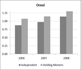
Economies of scale are given by the sum of the production elasticities. Figure 1 shows that in Tatarstan both organisational form operated at almost optimal farm size, e.g. constant returns to scale. The situation in Oreol was different as economies of scale fluctuated over time in that region suggesting that the forces for farm restructuring were much more pronounced than in Tatarstan. These results are also consistent with the restructuring process which occurred in Oreol after the breaking up of one of the large horizontally and vertically highly integrated structures in Oreol mentioned in Section 2.
Figure 1: Economies of scale by organisational form
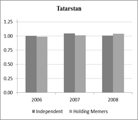
Source: own calculations
The majority of the parameter estimates for holding membership were not statistically significant implying that the production structures for group members and independent farms were rather similar. However, there is indication that holdings were less able to benefit from technical change than independent farms (amt < 0) and that the production possibilities were lower in holding members (am < 0). However, these results concern the parameter estimates only, the conclusions when comparing the production elasticities by farms may deviate[13]. Moreover similar elasticities in the groups might not indicate that marginal return are the same. In order to get more information on these issues we used the definition of elasticities as the ratio of marginal and average effect to take a closer look on the two components (Table 4a and b).
Because of the normalisation of variables, the means of the production elasticities for independent farms are exactly the same as the parameter estimates for the first order terms presented in Table 3. Morever, the calculations provide that almost all elasticites differ among the organisational forms. In both regions, holding members showed higher elasticities than independent farms. Only the production elasticities for capital were higher in independent farms. Despite the differences in farms size (see Section 2) the structure of production in both regions was rather similar among the organisational forms. This finds its expression in the mostly insignificant differences between average productivities. However, labour productivity in holding member were significantly higher than in independent farms. This corresponds to the release of labour by the mother company after a farms becomes a member of an holding.
Significant differences in production elasticities and insignificant results for average productivities already provide indication that the shadow prices will also differ among organisations. This conjecture is confirmed by the calculation. Consistent with the lower labour input in holding members, in both regions the marginal product of labour was higher in this organisation form than in independent farms. This result supports the often heard proposition that agroholdings are more profit-oriented; they release underemployed labour, and thus are fulfilling the social function of farms less satisfactory than independent agricultural enterprises.
The other results regarding the marginal products are less conclusive. In Tatarstan purchased inputs (capital, materials) received a higher remuneration in independent farms than in holding members. These results are consistent with the hypothesis that many independent farms may be subject to credit and/or liquidity constraints so that they are unable to acquire sufficient purchased inputs. Given the financial strength of the holdings the access to purchased inputs will be better implying a lower shadow price of these inputs. However, in Oreol the opposite effects were observed. Holding have higher shadow prices. The reason might be that because of the economic problems of one of the large holdings which finally led to restructuring among the holding (Chap. 2). Given this development it can be expected that high adjustment and transaction costs occur in the development and creation of new business relationships which also hamper the access of holding members of the markets for purchased inputs.
Table 4a: Marginal and average productivities by organisational form, Tatarstan
|
|
Production elasticities |
||||
|
|
Labour |
Land |
Capital |
Materials |
|
|
Independent |
0.066 (0.046) |
0.320 (0.039) |
0.208 (0.051) |
0.419 (0.075) |
|
|
Members |
0.126 (0.057) |
0.327 (0.033) |
0.075 (0.049) |
0.482 (0.065) |
|
|
t-Value |
-11.789*** |
-1.275 |
23.701*** |
-8.484*** |
|
|
|
Average productivities |
||||
|
|
Labour |
Land |
Capital |
Materials |
|
|
Independent |
1.132 (0.616) |
1.129 (0.572) |
1.434 (1.945) |
1.135 (0.606) |
|
|
Members |
0.913 (0.428) |
1.155 (0.604) |
1.121 (1.139) |
0.877 (0.462) |
|
|
t-Value |
3.386*** |
-0.407 |
1.552 |
4.034*** |
|
|
|
Marginal productivities |
||||
|
|
Labour |
Land |
Capital |
Materials |
|
|
Independent |
0.076 (0.080) |
0.361 (0.188) |
0.236 (0.146) |
0.441 (0.126) |
|
|
Members |
0.124 (0.082) |
0.373 (0.193) |
0.046 (0.079) |
0.412 (0.161) |
|
|
t-Value |
-5.490*** |
-0.565 |
12.626*** |
1.997** |
|
Notes: *;**, *** denote significance at the 10%, 5% and 1% level, respectively
Standard deviations in parenthesis
Table 4b: Marginal and average productivities by organisational form, Oreol
|
|
Production elasticities |
||||
|
|
Labour |
Land |
Capital |
Materials |
|
|
Independent |
0.121 0.080 |
0.093 0.171 |
0.195 0.076 |
0.569 0.140 |
|
|
Members |
0.150 0.080 |
0.170 0.167 |
0.253 0.071 |
0.588 0.153 |
|
|
t-Value |
-2.649*** |
-2.757*** |
4.518*** |
-1.814** |
|
|
|
Average productivities |
||||
|
|
Labour |
Land |
Capital |
Materials |
|
|
Independent |
1.136 0.701 |
1.265 0.914 |
1.288 1.247 |
1.169 0.746 |
|
|
Members |
1.445 1.019 |
1.392 1.110 |
1.192 1.112 |
1.107 0.441 |
|
|
t-Value |
-2.729*** |
-0.894 |
0.518 |
0.580 |
|
|
|
Marginal productivities |
||||
|
|
Labour |
Land |
Capital |
Materials |
|
|
Independent |
0.161 0.191 |
0.206 0.371 |
0.222 0.174 |
0.591 0.244 |
|
|
Members |
0.254 0.268 |
0.333 0.494 |
0.266 0.215 |
0.624 0.238 |
|
|
t-Value |
-3.052*** |
-2.164*** |
-1.644* |
-0.912 |
|
Notes: *;**, *** denote significance at the 10%, 5% and 1% level, respectively
Standard deviations in parenthesis
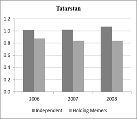
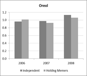
The parameter estimates were further used to calculate total factor productivity (TFP) as the main indicator or performance of the farms. We proceed by using the extension of the Diewert’s (1976) quadratic lemma by Caves et al. (1982). Within this context, input and output aggregates are calculated in relation to the mean of production and factor use which allow multilateral consistent comparison of total factor productivity. Given that TFP is defined as the ratio of an output and aninput index thus capturing the influence of scale adjustment and technical progress. Since the scale effect can be neglected (see Figure 1) it can be assume the TFP index measure gives information about technical progress only.
In Tatarstan TFP of independent farms grew over the whole period. Moreover, TFP was higher than in group members. TFP of business group members decreased, implying the agroholding members were falling behind the independent farms. This results is consistent with the observation that holding in Tatarstan experienced difficulties with agricultural production (see Chap. 2). In Oreol the independent farms experienced the same development as in Tatarstan. The group members in Oreol also fall behind, however, the experienced an increase in TFP. The results regarding TFP suggest that independent farm appeared to be better positioned than group members to benefit from technological change.
Figure 2: TFP level and development by organisational form (mean = 1)
Source: own calculation
Production risk and Inefficiency
The parameter estimates of the risk function provide that on average the general production condition over the year were quite similar. Most of the parameters capturing the impact of input on risk were significant and generally positive, e. g. risk increasing. Only land input in Tatarstan was risk reducing. Although the data set was not detailed enough to consider the impact on risk appropriately, these results provide that risk management practices seemed to be underdeveloped in both regions. Agroholding membership appeared to risk increasing. This result is consistent with the more intense use of purchased inputs in this organisational structure[14].
The regression results for the inefficiency functions varied considerably between the regions. In Oreol inefficiency did not play a role at all, e.g. su was very small. This does not indicate that all farms were at their production frontier, rather it just means that there were no pronounced efficiency differences among the farms and all inter farm variation was captured by the two-sided error term. In Tatarstan, in contrast, inputs affected efficiency considerably. Land and capital increased efficiency, while materials decreased efficiency. Moreover, agroholding membership had a huge negative impact on inefficiency. Given the structure of the inefficiency function it can concluded that the holding effect drives the whole inefficiency towards zero. This result might be due to the large differences in farm size between agroholding members and independent farms and the relative small number of group members in the sample.
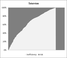
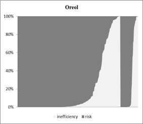
Using the
decomposition ![]() the share of risk and
inefficiency on total output variance can be seen from Figure 3. Basically, the
Figure confirms the implications already derived the discussion of the
parameter estimates: In Oreol production risk is the most important source of
farms’ output variation. This holds for both types of organisational forms. In
Oreol production risk accounts for all of the farms’ output variation. This is
simply due to the fact that no inefficiency could be estimated. Risk is also an
important source of output variance for independent farms. However, in this
region inefficiency has a considerably larger share on output variation than in
Oreol.
the share of risk and
inefficiency on total output variance can be seen from Figure 3. Basically, the
Figure confirms the implications already derived the discussion of the
parameter estimates: In Oreol production risk is the most important source of
farms’ output variation. This holds for both types of organisational forms. In
Oreol production risk accounts for all of the farms’ output variation. This is
simply due to the fact that no inefficiency could be estimated. Risk is also an
important source of output variance for independent farms. However, in this
region inefficiency has a considerably larger share on output variation than in
Oreol.
Figure 3: Share of production risk and technical inefficiency on output variance

Source: own calculations
Note: shaded areas denote the agroholding members.
5.3 Variance decomposition
In this section we discuss how the parameter estimates affect the contribution of production, risk and inefficiency to the variance of inputs. (Table 5).
Table 5: Statistical indicators for mean production, risk, and efficiency
|
|
Tatarstan |
Oreal |
||
|
|
Indepen |
Holding Members |
Indepen |
Holding Members |
|
Mean production |
55.1% |
66.5% |
40.5% |
80.3% |
|
Land |
71.4% |
95.3% |
38.1% |
56.2% |
|
Land productivity |
28.6% |
4.7% |
61.9% |
43.8% |
|
Risk |
24.1% |
30.2% |
51.2% |
12.3% |
|
Inefficiency |
20.8% |
3.3% |
8.4% |
7.3% |
Note: Mean production was decomposed using equation (1). The contributions are calculated in relation to the total variance of mean production.
Source: Own estimations.
In both regions mean production was the main source of output variance. This indictor was further separated into the variance of farm size measured by land and the variance of land productivity. The results were rather different between regions as well as organisational forms. The holding member in Tatarstan the almost the whole variation was due to farm size, land productivity was very similar. One reason might be that the group members because of their size are focussing on crop production. The other farms (independent in Tatarstan as well as independent and holding members in Oreol) showed a more balanced contribution of land input and land productivity.
Moreover, from Table 5 it followed that the variance of the risk function contributes significantly more to output volatility than efficiency in both regions and for both organisational forms. Thus, policy measures aiming at increasing productivity of farms might not be the best choice, since the increase of efficiency might have only a relatively small impact on output variability. More beneficial would be to assist farm in adopting risk management practices since decreasing production risk would have a high impact on production volatility. This conclusion is fortified by the finding in Figure 3, where it was shown that for most farms risk is much more important than inefficiency. Moreover, the parameter estimates in Table 3 revealed that the mechanism of risk management appear to be low developed.
6 Conclusion and interpretation
First, we investigated product prices and production in terms of average productivities. Our data set allows conducting corresponding analyses for grain and milk. Marked differences between organisational structures are not observable, neither for prices nor for partial productivities.. This indicates that members of a business group are obliged to use the channels offered by the holding company, however, they are paid a price oriented towards the average price paid in the regions and benefit from a reduction of transaction cost.
Second, the determinants of production variance were estimated using a risk production function with an inefficiency component. The parameter estimates confirm that all effects are highly important. Moreover, agroholding membership significantly affects the production structures. The results support the view that these companies in Tatarstan have a better access to purchased inputs and use them more intensively than independent farms. Labour input is lower in holding members suggesting that this group pays less attention to the social function of farms in rural areas. In addition, both organisational forms seem to operate under constant returns to scale. Technical change was strongly biased, e. g. labour and land using as well as capital and material input saving. The affect in Oreol for similar, however, not as expressed. This can be due to the fact that holdings in Oreol were created under control of the Oblast government which is not only interested in the economic but also social function of farms. Almost all inputs except land had a risk increasing effect. This indicates the farms do not apply management techniques in noteworthy extend. Consistent with the more intense use of inputs, agroholding membership appears to have a higher (generic) production risk. For inefficiency we found almost inverse results. Generic inefficiency in agroholdings is significantly smaller than for independent farms.
The estimates provide further that risk is of higher relevance for the variation of production than inefficiency. Moreover, for independent farms risk and inefficiency explain about the same amount of production variance than technology differences. Thus, risk and internal transaction costs appear to be much more important than market inefficiencies. The latter conclusion is also relevant for holding members. However, it has to be emphasised that compared to independent farms these variances are on a relatively low level indicating that differences in technology are more pronounced in this group.
In sum the results suggest that all three components, e. g. production risk, conditions on the product market and inefficiency, significantly affect agricultural production. Thus, for improving the conditions, agricultural policy is required to tackle all the issues using a mix of appropriate policy measures. However, the focus should be on the adoption of risk management techniques to reduce the volatility of output. The conclusion holds for both organisational forms. Relatively stable outputs are one necessary condition for a stable and healthy financial situations, these are in turn a precondition for investment and purchases of material inputs. Thus appropriately designed political support could induce positive feedbacks effects which lead to sustainable developments in Tatarstan and Oreol agricultural sectors.
Literature
Azzalini, A. (1985): A class of distributions which includes the normal ones. Scandinavian Journal of Statistics 12, 171-178
Azzalini, A. (1986). Further results on a class of distributions which includes the normal ones. Statistica 46, 199-208
Bokusheva, R. and Hockmann, H. (2006): Production risk and technical inefficiency in Russian agriculture. European Review of Agricultural Economics 33: 93-118.
Caves, D. W., Christensen, L. R., and Diewert, W. E. (1982): Multilateral comparisons of output, input, and productivity using superlative index numbers. The Economic Journal 92: 73-86
DeGroot, M. H. (1989): Probability and statistics. Addison-Wesley. Reading et al.
Hockmann, H., Bokusheva, R., Bezlepkina, I. (2009): Agroholding membership: does that make a difference in performance? Quarterly Journal of International Agriculture. 48 (1): 25-46.
Jondrow, J., Lovell, C. A. K., Materov I. S. and Schmidt, P. (1982): On the estimation of technical inefficiency in the stochastic frontier production function model. Journal of Econometrics 19: 233-38.
Just, R. E. and Pope, R. D. (1978): Stochastic representation of production functions and econometric implications. Journal of Econometrics 7: 67–86.
Koester, U. (2005): A revival of large farms in Eastern Europe? - How important are institutions? in: Colman, D. and N. Vink (eds.), Reshaping Agriculture's Contributions to Society. Proceedings of the Twenty-Fifth International Conference of Agricultural Economists 2003 in Durban, South Africa. Blackwell Publishing 2005, pp.103-114.
Kolesnikov, A. (2009): Ocenka finansovogo sostoyaniya agropromyshlennykh formirovanoniy (Assessment of the financial situation of agro-industrial formations), in: APK: ekonomika, upravlenie, Nr. 10, S. 60 – 63.
Kumbhakar, S. C. (2002): Specification and estimation of production risk, risk preferences and technical efficiency. American Journal of Agricultural Economics 84: 8–22.
Kumbhakar, S. C. and Lovell, C. A. K. (2000): Stochastic frontier analysis. Cambridge: Cambridge University Press.
Svetlov, N. (2009): Estimating Internal Transaction Costs: Case of Dairy Corporate Farms in Moscow Oblast of Russia. Agrarwirtschaft 58 (8): 346-353
Svetlov, N. and Hockmann, H. (2007): Long-term efficiency of the Moscow region corporate farms during transition (evidence from dynamic DEA): "Economic transition in midlife: lessons from the development of markets and institutions", Conference of the Chinese Economists Society, May 11-14, 2007. Portoroz, Slovenia.
Voigt, P. and Hockmann. H. (2008): Russia's transition process in the light of a rising economy: Economic trajectories in Russia's industry and agriculture. European Journal of Comparative Economics 2 (5): 251-267
Wandel, J. (2010): Integrierte Strukturen im Agrar- und Ernдhrungssektor Russlands: Entstehungsgrьnde, Funktionsweise, Entwicklungsperspektiven und volkswirtschaftliche Auswirkungen". Habilitationsschrift. Martin - Luther - Universitдt Halle - Wittenberg.
Appendix
A first order Taylor approximation of a product (p y) around the means of the variables (p0,y0) is given by:
![]()
Applying the definition of the variance provides:
![]()
Expanding the bracket and putting the expectation operator through provides:
 .
.
In this
expression we already simplified by using ![]() and
and ![]() . Applying the definition of the variance and covariance
yields:
. Applying the definition of the variance and covariance
yields:
![]() .
.
Putting the terms containing covariances into the function c(p,y) provides:
![]() .
.
[1] On this issue see for instance Kolnesnikov (2009), Wandel (2010) and Hockmann et al. (2009)
[2] The main difference to other regions was that in these the evolution of holding structures was initiated by the regional government, however, it was mainly a privately driven process like in Belgorod.
[3] There is no legal definition of an agroholding. Correspondingly, holding membership is not defined in official statistics, however, most analysis define these organisations using a definition provided by Ushativ as group of companies which are connected via asset and contractual relationships. This definition allows using a simple practical approach of defining group membership (Uzun): A farm is a member of an agroholding when the owner of a farm owns other farms as well. Since the eh classification was done using all agricultural enterprises in the Russian federation the identification of owner structures should be quite accurate. The available data provides only information whether a farms is a member of a business group but does not identify the business group itself.
[4] Svetlov (2009) and Svetlov and Hockmann (2007) investigated the role of external transaction cost in agriculture in Moscow oblast. Using a different approach (DEA) they also found that this cost significantly affects agricultural holdings.
[5] In the following, bold symbols indicate vectors or matrices; all other variables are scalars. Subscripts will be omitted in order to improve readability.
[6] The assumption , e. g. sv = 1, results from the introduction of the idiosyncratic component into the risk function. Without this assumption, the model would not be identified.
[7] l is called the shape or skewness parameter, while s represents the variance or scale parameter or variance (Azzalini 1985 and 1986).
[8] The proportional shift is given by the Jacobian (J). The Jacobian has to be applied because of the transformation from e to y (DeGroot 1989). In the standard workhorse the Jacobian can be omitted because the differential is equal to one.
[9] Regarding curvature we restrict ourselves to the main diagonal of the Hessian matrix and implemented the “law of diminishing marginal returns” in order to reduce the computational burden. Due to this simplification the number of the curvature restrictions reduced from 15 to four for each new data set.
[10] The estimations were conducted using GAUSS and the CML procedure.
[11] Assuming a translog aggregator function, the result is a Tцrnquist-Theil Index. Basically, by this approach each observation is compared to the average in the sample.
[12] We omit a formal Wald test. First, given the significance of the parameters the result of the test is trivial. Second, the logic behind testing a parameter or a group of parameters against the H0 Hyothesis would be to check whether a more restricted model could be used.
[13] This stems from the fact that the parameter capturing the cross effects have to be considered in the calculation.
[14] A more intense use of material inputs implies lower partial productivity of material inputs in agroholding members. See Tables 4 for more information.
Назад в раздел